Behavioral Cloning and Interactive Imitation Learning
Course notes on behavioral cloning and interactive imitation learning, covering loss functions, distribution shift (DAgger), and key theoretical foundations.
Mainly speaking, this is a course note on behavioral cloning and interactive imitation learning, which are two important techniques in the field of imitation learning. The content is based on the lecture slides provided by the course instructor, Daniel Brown.
Imitation Learning
Can also be called as “Learning from Demonstrations”. The main idea is to learn a policy that can mimic the behavior of an expert demonstrator.
Behavioral Cloning
Behavioral cloning is a simple approach to imitation learning, where we treat the problem as a supervised learning problem. We collect a dataset of state-action pairs from the expert demonstrator, and then train a policy to predict the action given the state.
Below we define two common loss functions for behavioral cloning:
The first is a cross-entropy loss for discrete action spaces:
\[\ell(\pi, s^{*}, a^{*}) = -\log \pi(a^{*}\mid s^{*})\]The above formula is a per-sample loss. In reality we use Monte Carlo estimation to compute the average loss over a batch of samples:
\[\mathcal{L}(\pi) = -\frac{1}{N}\sum_{i=1}^{N} \log \pi(a_i^* \mid s_i^*)\]Why discrete?: Cross-entropy requires \(\pi(a \mid s)\) to be a probability of taking action \(a\). This works when the action space is discrete, so that the policy outputs a probability distribution over actions (e.g., via Softmax). However, for continuous action spaces, we cannot directly apply cross-entropy loss, because the number of possible actions is infinite, and we can NOT assign a probability to each individual action.
However, using cross-entropy loss to model continuous action spaces is still possible if we model the policy as outputting distribution parameters (e.g., a Gaussian policy, which parameterizes the mean \(\mu\) and variance \(\sigma^2\)), and use negative log-likelihood as the loss function.
The second is a mean squared error (MSE) loss for continuous action spaces:
\[\ell(\pi, s^{*}, a^{*}) = \|\pi(s^{*}) - a^{*}\|^{2}\]where \(\pi(s^{*})\) is the action \(a\) predicted by the policy given the state \(s^{*}\), and \(a^{*}\) is the action taken by the expert demonstrator.
Now the task becomes simple: minimize the loss function over the dataset of state-action pairs collected from the expert demonstrator.
Pros and Cons of Behavioral Cloning
Below I list some of the pros and cons as far as I understand:
Pros:
- Simple and easy to implement.
- Can be effective when the expert demonstrations are of high quality and cover a wide range of states.
Cons:
- Covariate Shift: The distribution of states encountered by the learned policy may differ from the distribution of states in the expert demonstrations, leading to compounding errors.
- Compounding Errors: Small errors in the learned policy can lead to states that were not seen in the training data, which can further degrade performance.
Here, compounding errors could be the most obvious issue. As the learned policy ONLY sees the right action for the states from the demonstrations, it may not know how to recover from states that are not visited in the demonstrations. As the policy keeps rolling out, small errors happen and accumulate, which gradually shifts the state toward something the agent is not aware of, finally triggering a complete failure (e.g., crash on a tree in an autonomous driving scenario).
Behavioral Cloning from Observation (BCO)
Behavioral Cloning from Observation (BCO) is a variant of behavioral cloning where the agent learns to imitate the expert’s behavior using only state observations, without access to the expert’s actions. The main idea is to first learn an inverse dynamics model that can predict the action taken by the expert given two consecutive states, and then use this model to generate pseudo-action labels for the state observations.
Inverse Dynamics Model
This is a model that predicts the action taken by the expert given two consecutive states.
\[(s_t, s_{t+1}) \rightarrow a_t\]BCO is essentially a meta-algorithm to perform imitation learning when we only have access to state observations. Below is its pseudocode:
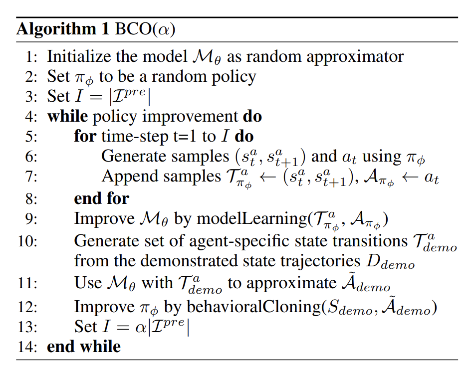
It can be a bit confusing. Let me clarify:
- At the start, parameters of the two models (the policy and the inverse dynamics model) are randomly initialized.
- length \(I\) is set to the number of demonstrations.
- inverse dynamics model is trained on the policy’s own experience (i.e., the state-action-next-state pairs collected by rolling out the current policy).
- Use the trained inverse dynamics model to predict the actions for the expert demonstrations.
- Train the policy using the demonstrated states and the predicted actions.
- Set the length
I=\alpha |L|, where|L|is the number of expert demonstrations. - Repeat steps 3-6 until convergence.
But it is also worth noting that, in practice, inverse dynamics model is often trained initially on a small amount of random exploration data in the target environment, before the main loop starts. This can help the model learn how the environment dynamics work, which can lead to better action predictions.